Access Geodata from the Web
Prof. Francesco Pirotti PhD <francesco.pirotti@unipd.it>
02 October, 2025


Exercises overview
- Exercise 1 - Download DEM and analyse terrain surface height values.
- Exercise 2 - Download and style multi-temporal rainfall rasters.
- Exercise 3 - Find new human settlements using lights visible from space.
- Exercise 4 - Styling a raster from color look-up tables.
The following handout gives instructions on how to access and download geospatial data from the web with different means:
The objective is to be able to hunt for geospatial data for your future projects, including the project required for passing the exam.
Downloading geospatial data from web providers
An internet portal that provides several geospatial datasets for downloading is usually called a “Catalogue”. Finding catalogues can be as easy as search using a search engine (e.g. Google), but sometimes require further investigation. In the next session some examples of web portals providing geospatial data with global, national and regional scales.
Global Datasets
GENERAL COLLECTIONS
Natural Earth Data
Free vector and raster map data at 1:10m, 1:50m, and 1:110m scales
Essential Climate Variables
GCOS Essential Climate Variables (ECV) Data Access Matrix
https://www.ncdc.noaa.gov/gosic/gcos-essential-climate-variable-ecv-data-access-matrix/
GEOSS portal
http://www.geoportal.org/ Geoportal allows to search for both downloads and W(FCM)S services (see section “Online web mapping services WMS / WCS / WFS”)
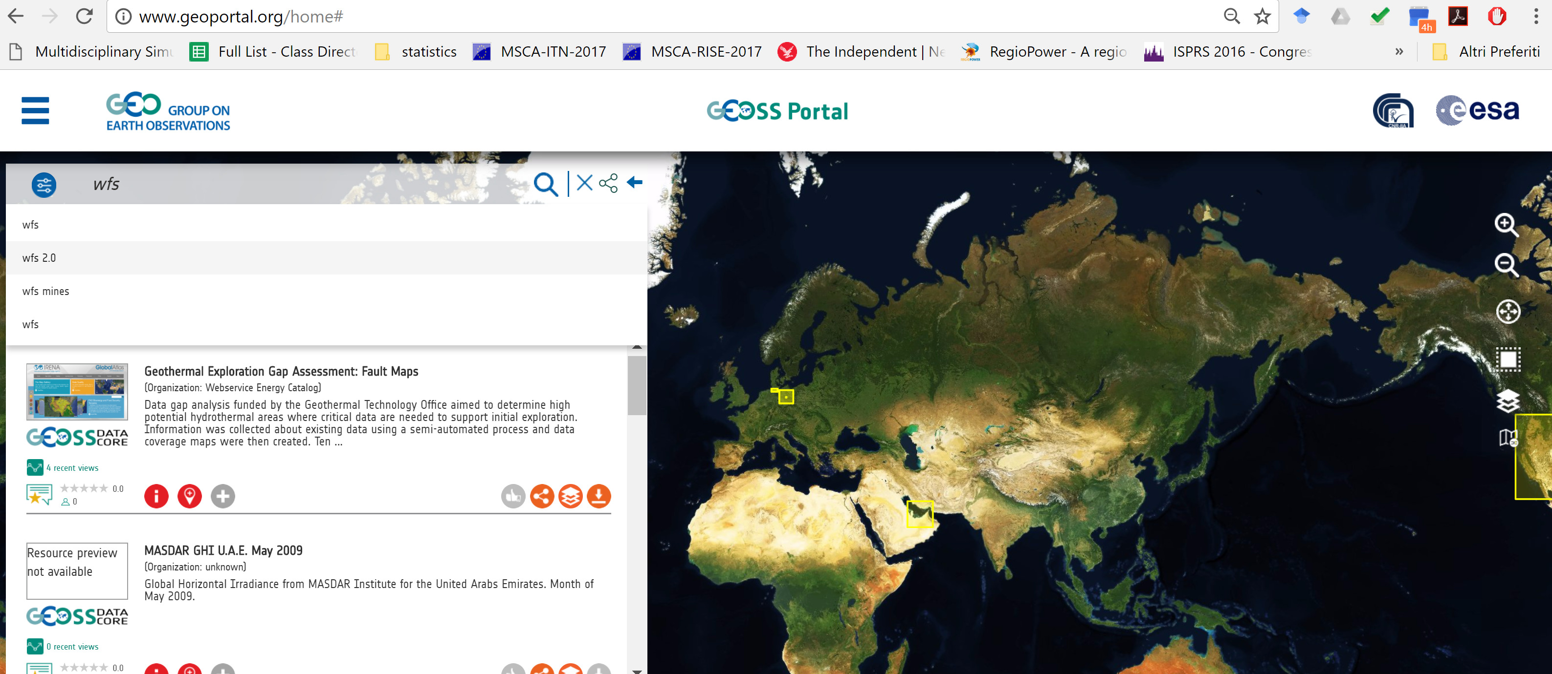
There are many options for filtering data. Not all data links are “live”, some links do not work, so it requires some searching for data.
COPERNICUS DATASPACE

COPERNICUS Services
https://dataspace.copernicus.eu/
Satellite data from the European Copernicus Programme:
https://dataspace.copernicus.eu/browser/
Also available on Wekeo - following link with layers of interest for agriculture, forestry and environmental sciences: https://wekeo.copernicus.eu/
e.g. predicted fire danger from climate models, Surface Soil Moisture at 1 km resolution,
Tree Canopy Cover and leaf type (broad-leaves vs conifers) at 10 m
CLMS = Corine Land Monitoring Service - Land Cover classes at 100 m resolution up until the year 2018 link - then available at 10 m! See below. NB - more spatial resolution but lower “semantic resolution” - compare legends.
Land Cover at 10 m resolution
Land cover maps, tree density, crop types…
Corine Land Cover Plus - 10 m

========================
COMPARE WITH…

Crop Types at 10 m resolution

Others
Check the many land cover here!
USGS: EarthExplorer
USGS EarthExplorer https://earthexplorer.usgs.gov/ provides raster data from satellite and airborne missions. Some missions provide a raster of height values (DEM - digital elevation model). In the following tutorial we will learn how to download a digital surface model (DSM) from the SRTM which differs from a digital terrain model (DTM) as the DSM values include heights of buildings and trees, whereas the DTM values are of the bare terrain.
In the following exercise we will learn how to get two DSM rasters from two different sensors,
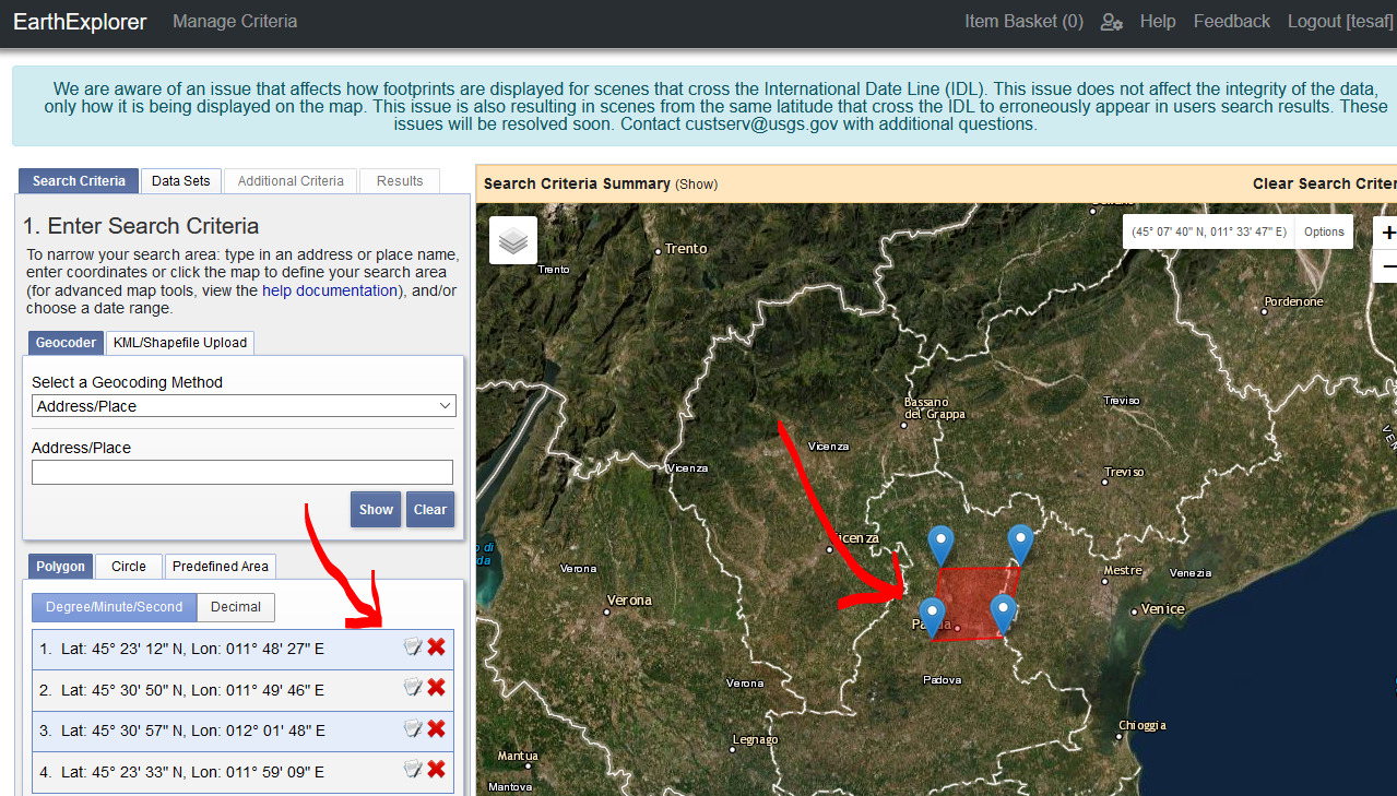
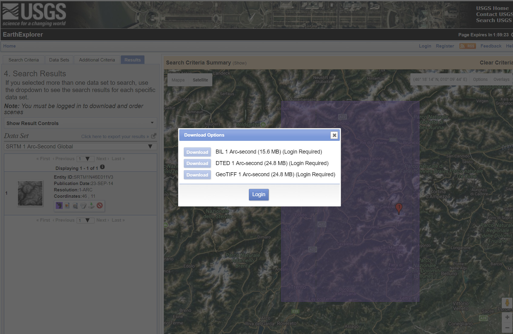
- Create a user profile by registering from https://earthexplorer.usgs.gov/
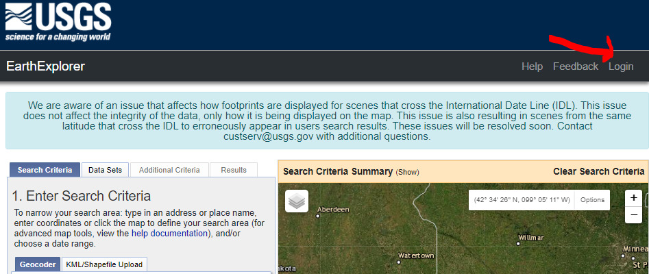
After registration proceed to login https://earthexplorer.usgs.gov/ with your registration credentials (username and password) by clicking “login” (see image above)
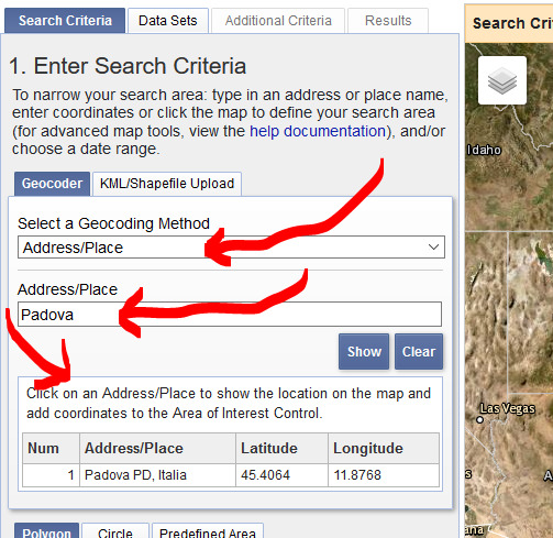
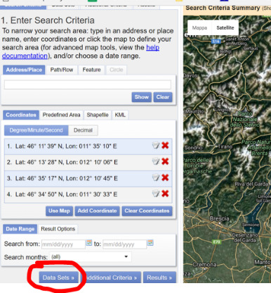
Identify your area in the map. There are several ways to do this:
Search by address / place (e.g. select “AddressPlace” and select Padova like the image on the right) NB this is available only if you are logged in!
Click the map directly to create a polygon or a point defining your area of interest like in the image below. You can remove polygon points on the table that appears or you can drag the points with the mouse to change the area.
- At the bottom of the page, click on “datasets” (in some cases you can choose to select a certain time window – that’s in case of multitemporal datasets)
- In the input space of “Data Sets Search” type “SRTM” – you will see the product that you can select by clicking the checkbox
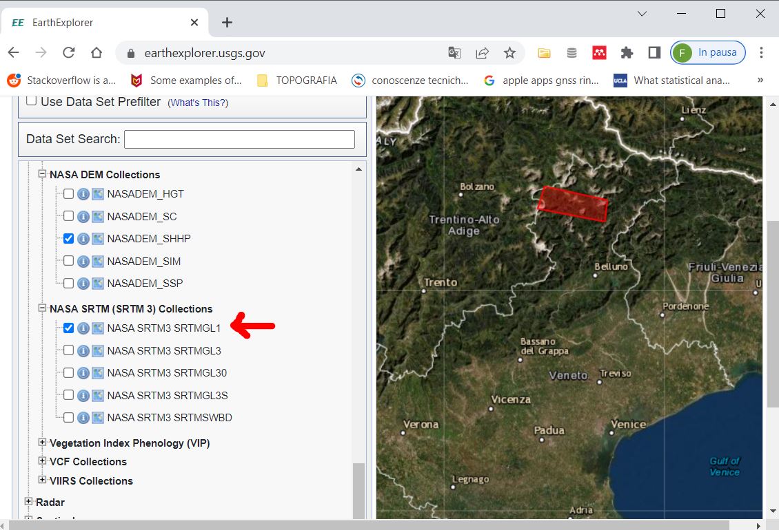
- All SRTM products intersecting your area will appear – for each product you can select from the toolbar the following (from left to right – see image below)
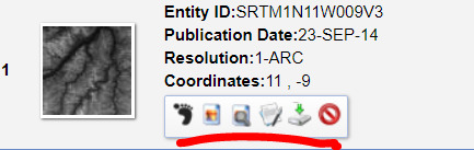
Show footprint
Show preview on map
Browse data
Show metadata
Download.
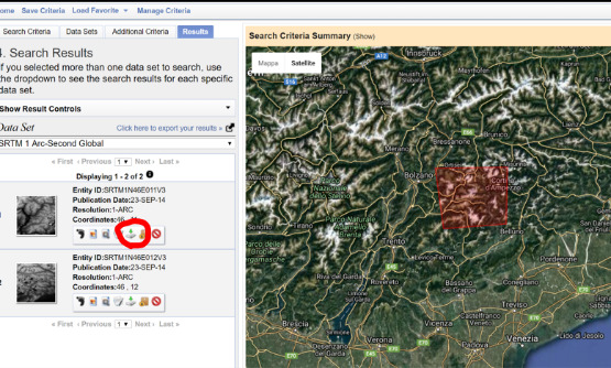
- You can choose from three different raster formats, QGIS is able to read all of them (more on Raster Formats @ http://www.gdal.org/formats_list.html )
- Load the file in your QGIS project –CRS of this file is 4326 (geographic latitude and longitude) – check handout on coordinate reference systems for more info in CRS.
Exercise 1
Exercise: download DEMs and analyse differences: with the procedures above download any two elevation datasets from the EarthExplorer portal and self-assess if you know how to answer the following two questions: - what are the two spatial resolutions? - compare differences in elevations of the two DEMs using the raster calculator in QGIS and style the map. What are the minimum and maximum values of the differences?
FAO: GeoNetwork
http://www.fao.org/geonetwork/srv/en/main.home
Excellent source of global and agricultural and environmental data
Exercise 2
Search for “rainfall African Water Resource Database” keywords and download rainfall data for Africa in two time windows, e.g. “APRIL 1ST-DECADAL SHORT MEAN RAINFALL”. This is Arc/Info Binary Grid.adf format (click link for more info). Style the map using QGIS. NB: the CRS (coordinate reference system) of this map is not known. Apply the same color scale to compare the two rasters.
United Nations - UNEP
Exercise 3
Find new human settlements using lighting visible from space. The Landsat satellite records (also) night-time imagery allowing to monitor human settlements using visible lights from space (~700 km from the Earth surface). Search and download “Nightlights” from two dates and use raster calculator to detect new human settlements in the most recent date. Try to come-up with mathematical expression to reach that objective. You can find a hint here - but try yourself first!
Marine Regions web services
Borders of world countries and other global data: https://geo.vliz.be/geoserver/MarineRegions/wfs
Google Earth Engine
Google Earth Engine is and advanced portal for processing satellite imagery and other geospatial big-data online through their map-reduce paradigm. You can put your hands on many datasets, process them and even download results or any intermediate data your produce – with limitations on the size of the data you can download. Coding is required (Javascript language through their online https://code.earthengine.google.com/ or Python through Jupyter notebooks). Welcome to coding/programming if you want to dive deeper in more advanced GIS.
SPECIFIC topics
Night lights map
https://eogdata.mines.edu/products/dmsp/ in this page you can download maps of night lights.
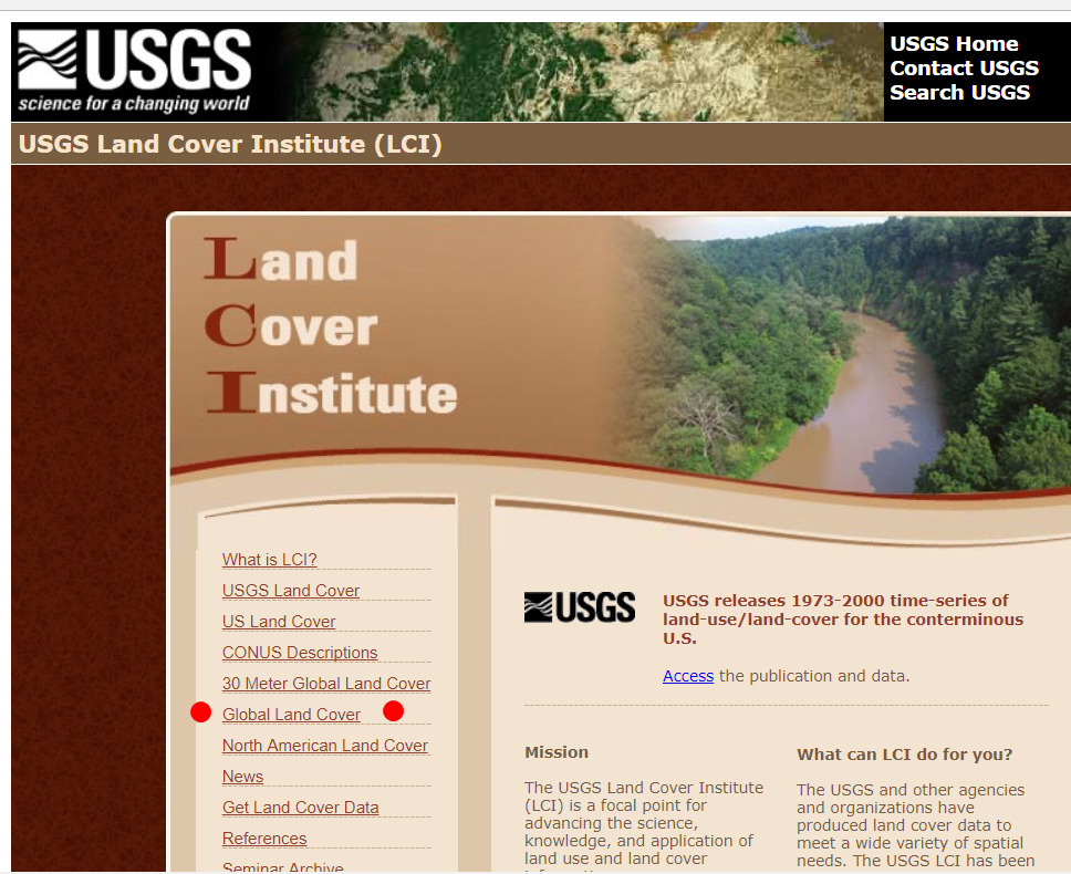
USGS: Land-cover
https://landcover.usgs.gov/ at link “Global Land Cover” (see image below) you will find a link to European Space Agency (ESA) datasets, see next section.
At link “30 meter Global Land Cover” also an interesting set of data for further GIS analyses (https://landcover.usgs.gov/glc/ ).
ESA: Land-cover
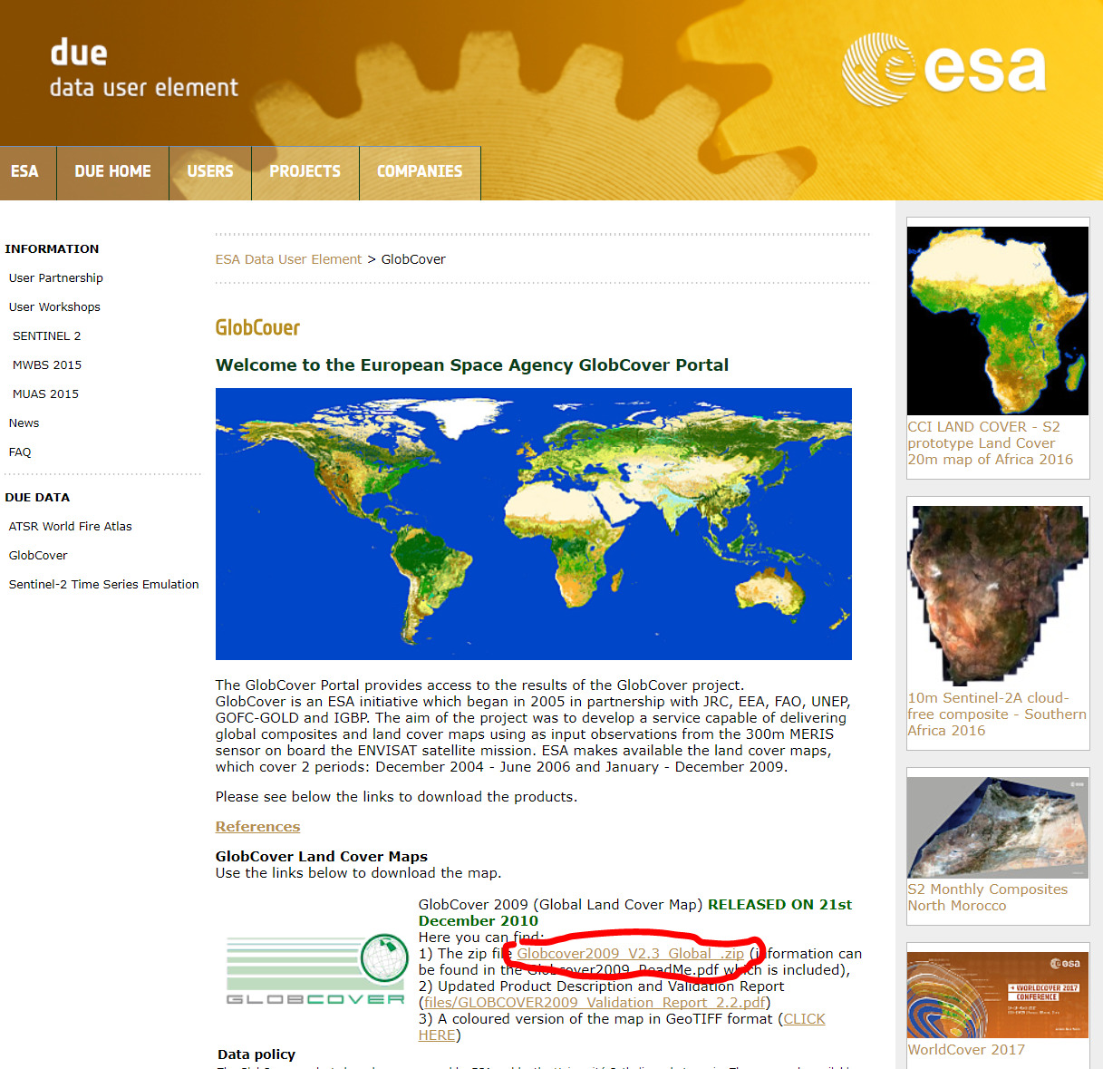
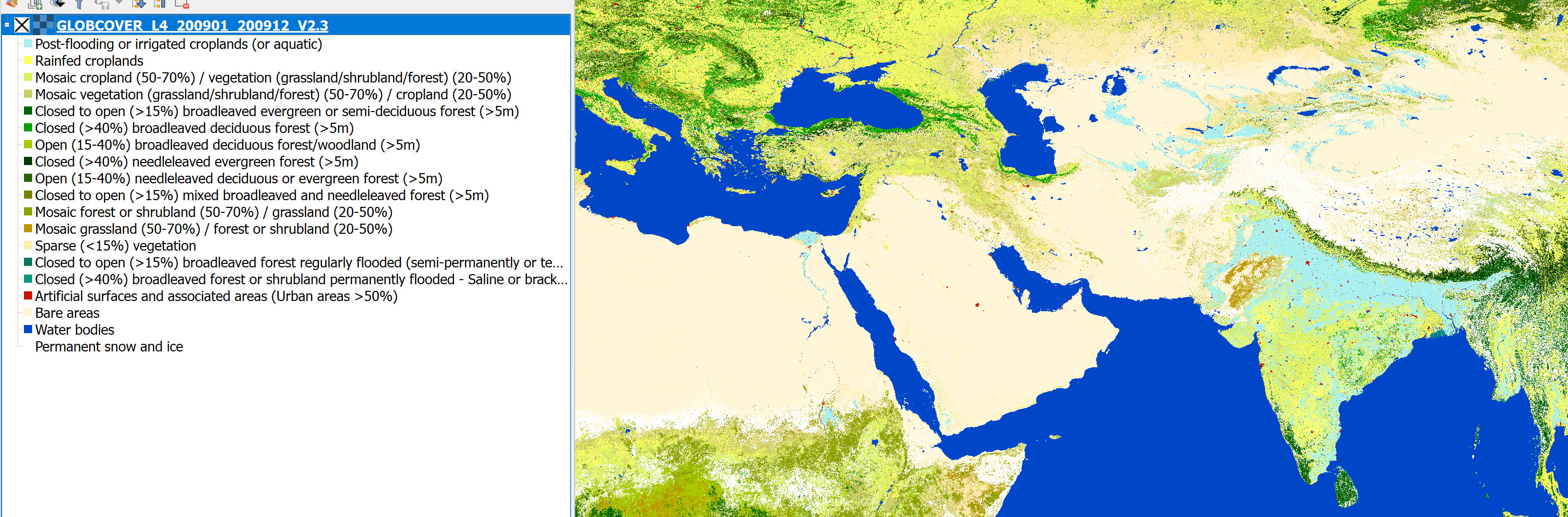
Exercise 4
Styling exercise with ESA GlobCover
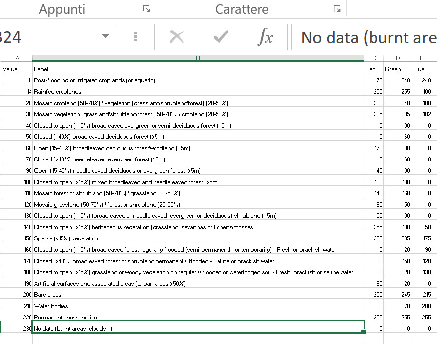
When you open with QGIS the GeoTIFF file, you only see numeric values of
the single cells. Each cell value corresponds to a legend
label. The label is found in the MS Excel file that is distributed
with the dataset. In this exercise you will learn how to create a
legend file to style the layer automatically.
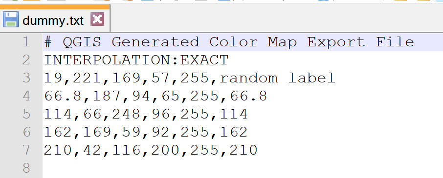
We can style the layer by right-click “Properties” and go the the
“style” dialogue, but it would take a long time to enter all values
by hand. Let’s do a trick: save a dummy legend,
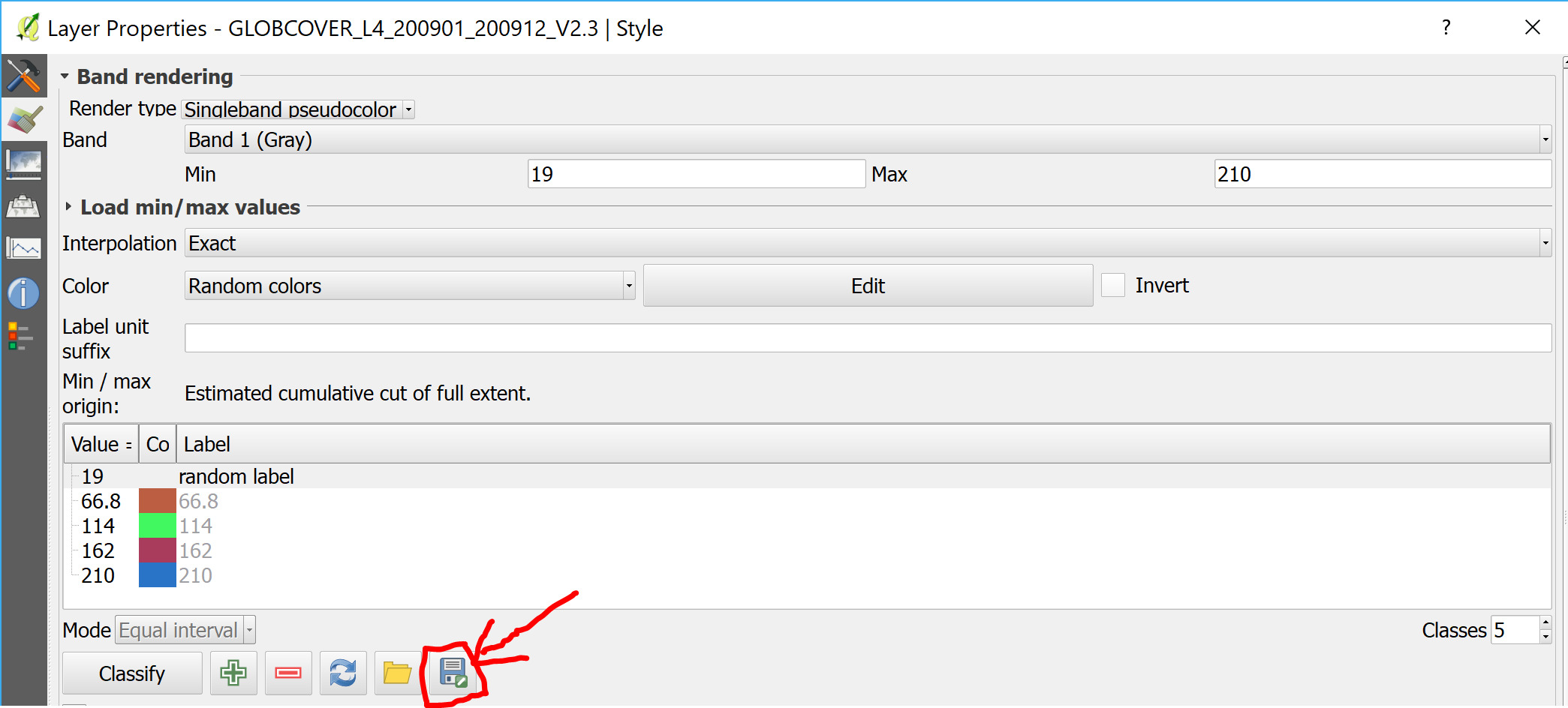
and then use a text editor to check format
Steps:
- In MS Excel in the legend file information change columns to mirror the above table
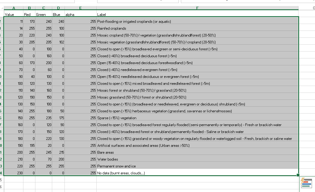
- Select (as image above) and copy/paste to the text file
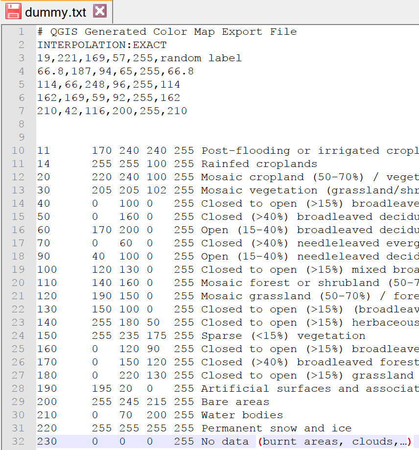
- Make sure to change column separators to correct ones (commas)
– a “find and replace” should work on any text editor. The
final result should be like the image below.
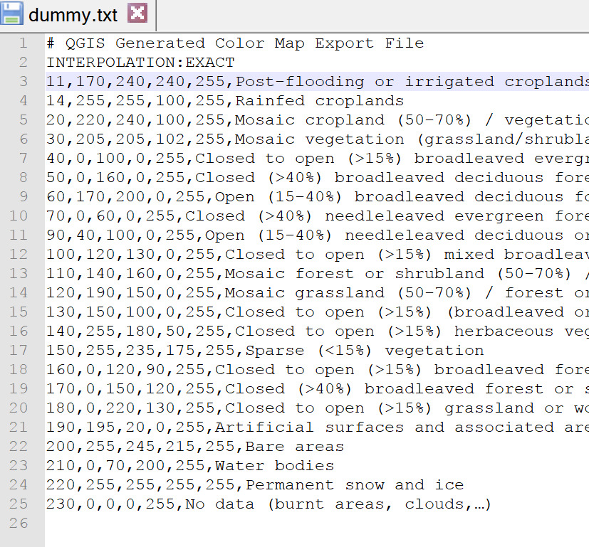
- Open the style dummy.txt that you modified
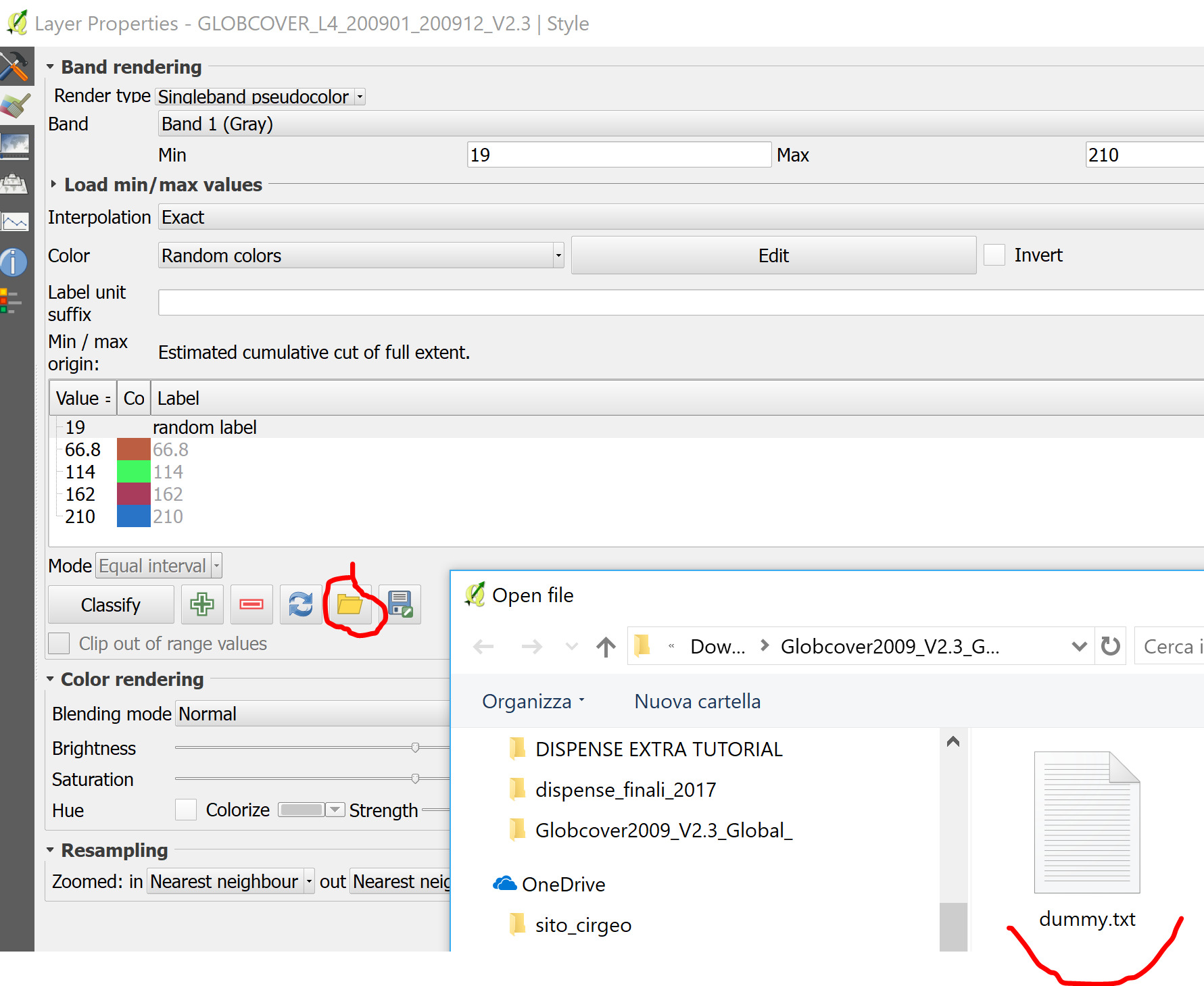
- You will get a correct legend
Forest Global Maps
University of Maryland’s Global Land Analysis and Discovery lab has two interesting datasets.
Forest Cover (with Gain and Loss from 2000) LINK HERE!!
Forest height - this is and estimation using remote sensing and GEDI laser altimeters data LINK HERE!!
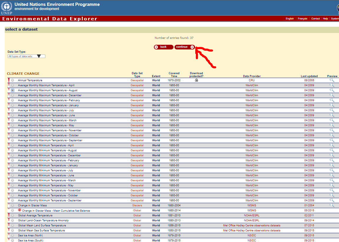
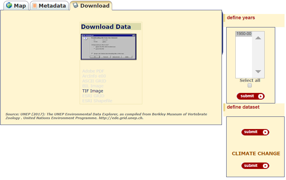
Climate WC v1
WorldClim is a set of global climate layers (gridded climate data) with a spatial resolution of about 1 km2. These data can be used for mapping and spatial modelling, and multi-criteria analysis (see the dedicated tutorial). http://worldclim.org
From the Google Earth Engine Catalogue description:
WorldClim V1 Bioclim provides bioclimatic variables that are derived from the monthly temperature and rainfall in order to generate more biologically meaningful values.
The bioclimatic variables represent annual trends (e.g., mean annual temperature, annual precipitation), seasonality (e.g., annual range in temperature and precipitation), and extreme or limiting environmental factors (e.g., temperature of the coldest and warmest month, and precipitation of the wet and dry quarters).
WorldClim version 1 was developed by Robert J. Hijmans, Susan Cameron, and Juan Parra, at the Museum of Vertebrate Zoology, University of California, Berkeley, in collaboration with Peter Jones and Andrew Jarvis (CIAT), and with Karen Richardson (Rainforest CRC).
Climate WC v2
WorldClim version 2 is a set of global climate layers (gridded climate data) with a spatial resolution of about 1 km2. These data can be used for mapping and spatial modelling, and multi-criteria analysis (see the dedicated tutorial). https://worldclim.org/data/worldclim21.html
For the GIS courses, the bioclimatic variables have been added to a Web Coverage Service (WCS - see dedicated section on how to load WCS services in your GIS here)
Right click this link and “copy link” to get the WCS address for WorldClim2 to add to your QGIS.
NB as readme.txt file states “
This is WorldClim 2.1 (January 2020) downloaded from
http://worldclim.org They represent average monthly climate data for
1970-2000.
The data were created by Steve Fick and Robert Hijmans
You are not allowed to redistribute these data
” Therefore please only use them for educational purposes and do not
redistribute data in any way.
Soil Carbon
From the website: “SoilGrids and WoSIS Soilgrids is a system for digital soil mapping based on a global compilation of soil profile data (WoSIS) and environmental layers. Read about the SoilGrids and WoSIS projects on isric.org” https://www.isric.org/explore/soilgrids
Precipitation: CHIRP
Researchers at Climate Hazard Center at University of California at Santa Barbara provide grid of 0.05° (around 5 km at the equator) with daily rainfall data https://chc.ucsb.edu/data/chirps
Regional datasets (Europe)
European Statistical (EUROSTAT)
https://ec.europa.eu/eurostat/web/gisco/geodata/reference-data
Provides vector data of boundaries and other important information at European and global level.
Example: https://ec.europa.eu/eurostat/web/gisco/geodata/reference-data/administrative-units-statistical-units/countries#countries20 and download boundaries in TopoJSON format. You can drag and drop the whole downloaded ZIP-file to QGIS! You will see that you can choose which files to open.
European Environmental Agency (EEA)
https://discomap.eea.europa.eu/Index/
Provides mostly WMS services (see section “Online web mapping services WMS / WCS / WFS”)
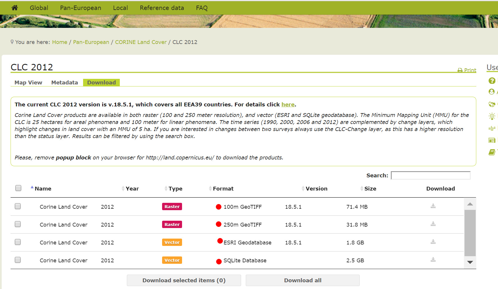
CORINE Land Cover
“An inventory of land cover in 44 classes, and presented as a cartographic product, at a scale of 1:100 000. This database is operationally available for most areas of Europe.”
You have 4 options for download
Raster (GeoTIFF) 100 m cell size
Raster (GeoTIFF) 250 m cell size
Vector model (ESRI Shapefile)
Vector model (SQLite Database).
Copernicus CORINE
The service below provides viewer and download capabilities, but you must register and login.
https://land.copernicus.vgt.vito.be/PDF/portal/Application.html
There is also a OGC services! (WMS/WFS/WCS)! You have to use the url
https://viewer.globalland.vgt.vito.be/geoserver/ows
and use the username and password in the credentials of QGIS. (see dedicated section on how to load OGC services in your GIS here)
Regional datasets (Italy)
ISTAT boundaries
Municipal boundaries updated every two years in ESRI shapefile at different detail. https://www.istat.it/it/archivio/222527
Trentino Aut. Prov.
LIDAR and Cartographic resources:
LIDAR from 2009 and 2014 https://siat.provincia.tn.it/stem/
Friuli Venezia Giulia
LIDAR and Cartographic resources:
https://eaglefvg.regione.fvg.it/eagle/main.aspx?configuration=guest
Lombardy Region
Veneto Region
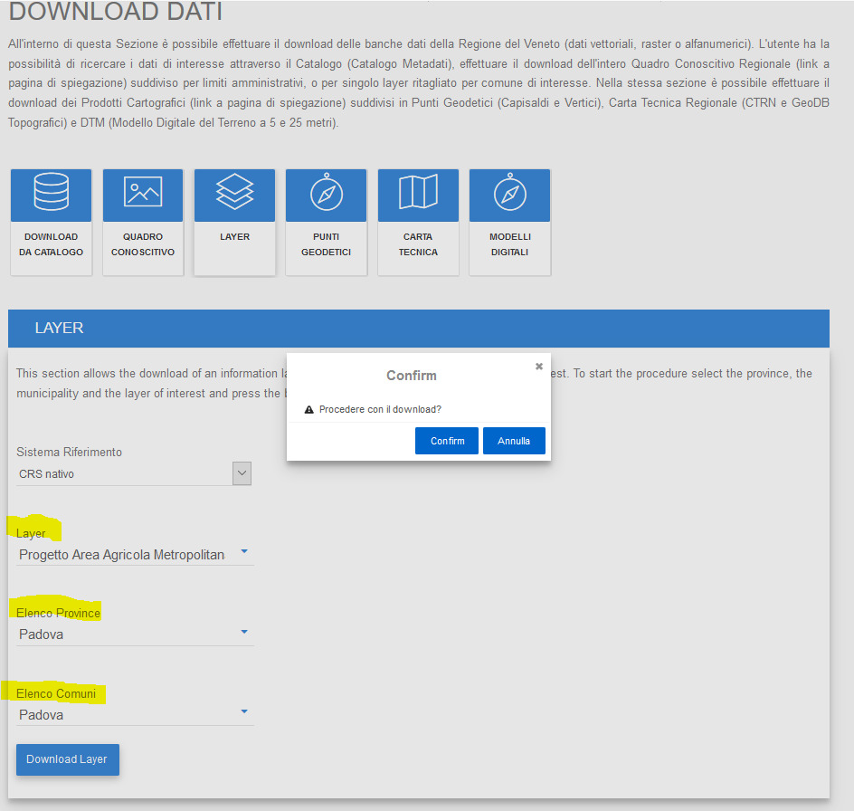
The Veneto Region portal - https://idt2.regione.veneto.it - provides downloading capabilities and also services (see chapter Online web mapping services WMS / WCS / WFS).
For downloading raster and vector datasets:
https://idt2.regione.veneto.it/idt/downloader/download
You can choose the CRS (see the handout on coordinate reference systems), and filter using the province and municipality of interest (e.g. Padova) – below and example for downloading the Urban Agricultural Areas.
If you want to mine for data using key-words, you can use the Catalog
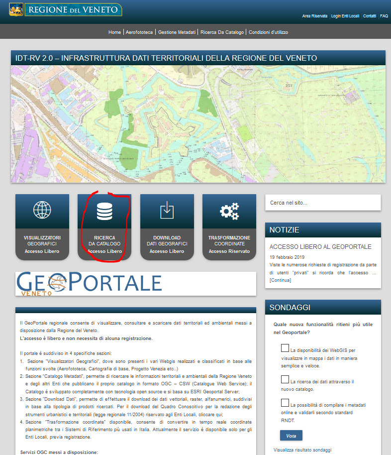
With key-words you can find both geospatial data and documents. If you want only geospatial data you can filter using only “Layers”
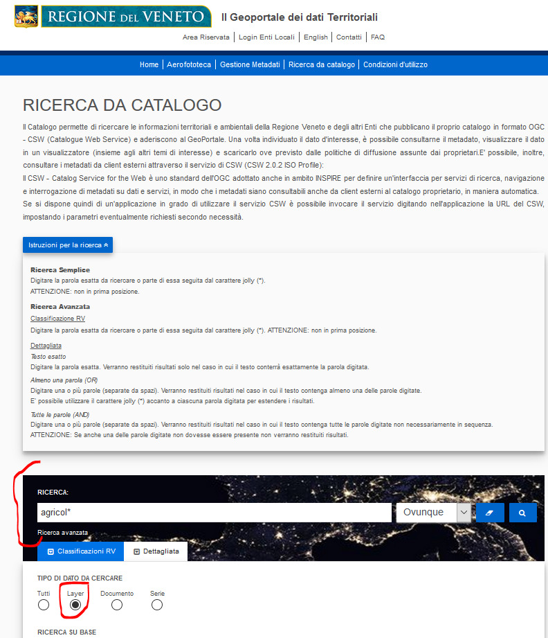
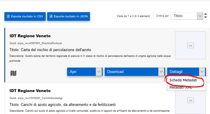
From results you can:
- Read metadata. Metadata keep all information that are not directly in the data – for example who is the owner, the date that data were acquired, copyright etc…
- You can download the layer for all the Region or for only a municipality or province.
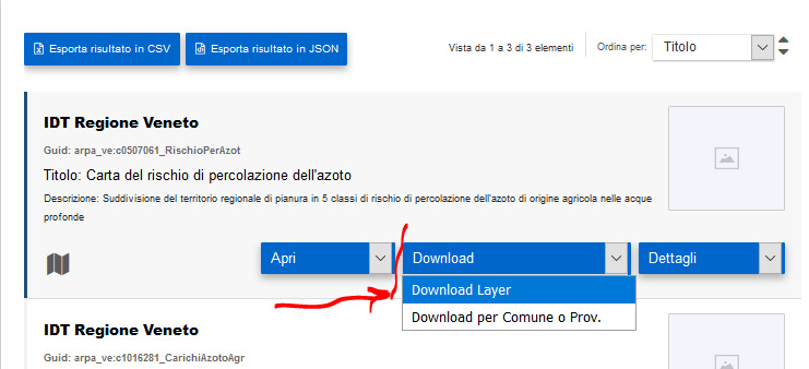
- Almost all data are available also via web services, check Online web mapping services WMS / WCS / WFS section below.
Online services WMS / WCS / WFS
These are online services providing access to the data for download or visualization. WMS is only for visualization, WCS and WFS are respectively for downloading data as well, for raster (grid) data and vector data respectively.
WMS – Web Mapping Services – see also tutorial
WCS – Web Coverage Services
WFS – Web Feature Services
There are many more services, which are standards defined by user community of the Open Geospatial Consortium (https://en.wikipedia.org/wiki/Open_Geospatial_Consortium ) - OGC. As a matter of fact these services have been recently referred to the term: OWS – Open Geospatial Consortium (OGC) Web Services.
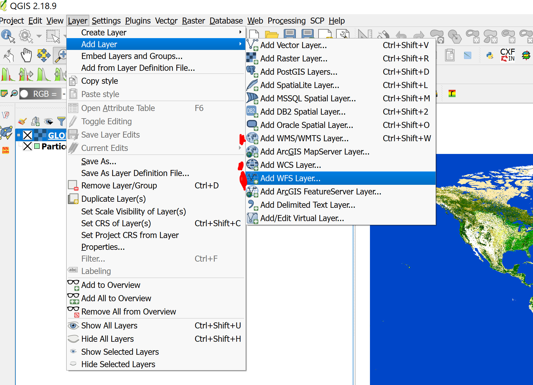
You access these data either from the menu bar, “Layer”“Add layer”
…or you can use the Data source manager by clicking the icon in the toolbar (see figure below).
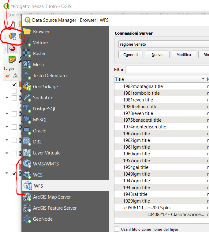
In all cases you will need to add a web address (URL) to the dialogue window. See next example and bottom of next section for some URL sources.
National Geo Portal – WFS services
http://www.pcn.minambiente.it/mattm/en/
Click “Services”Network Services - OGC”.
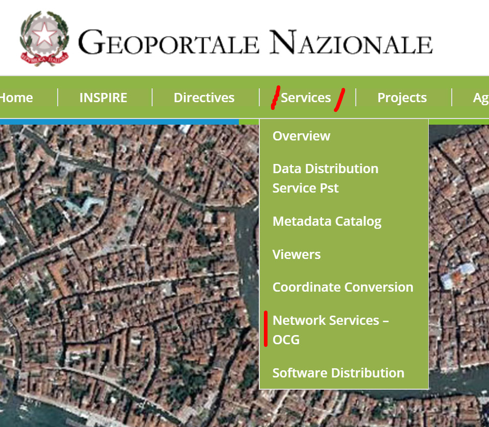
Select in the next page WFS Services
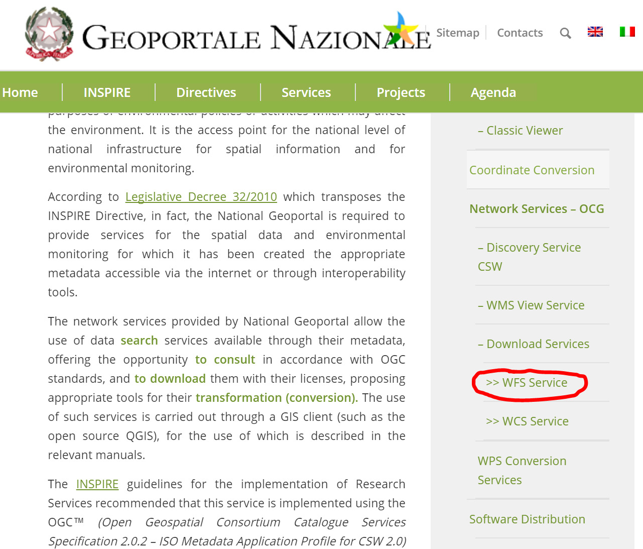
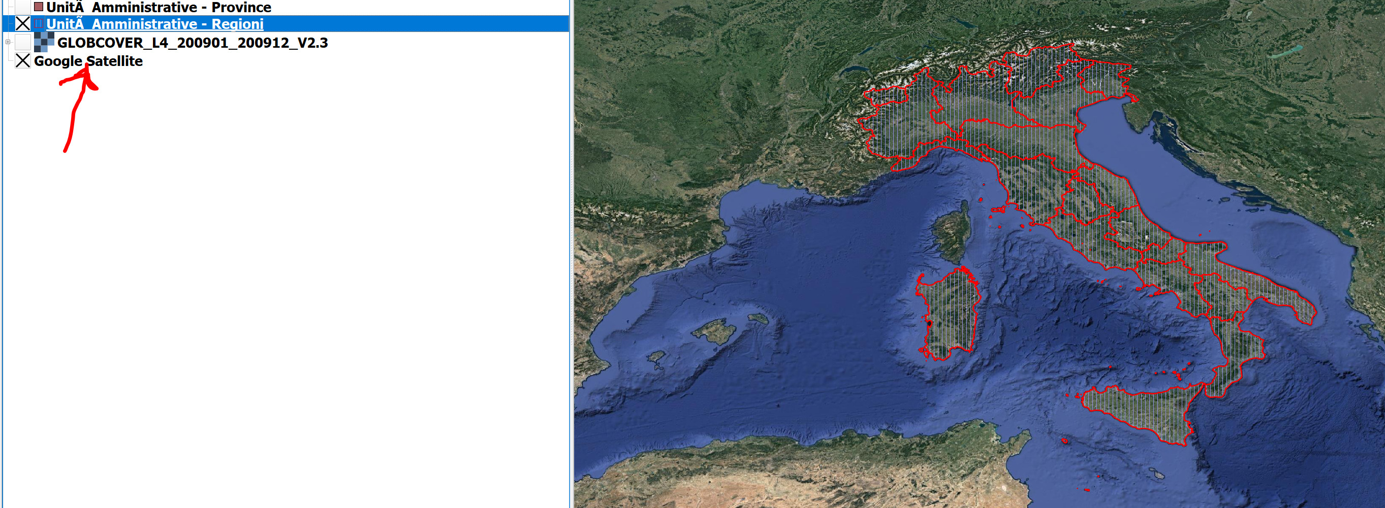
You will see a list of datasets, all have a URL address – we will “Copy URL” of the data we want. For example “Unità amministrative” is the border of municipalities in Italy (layer names are only in Italian).
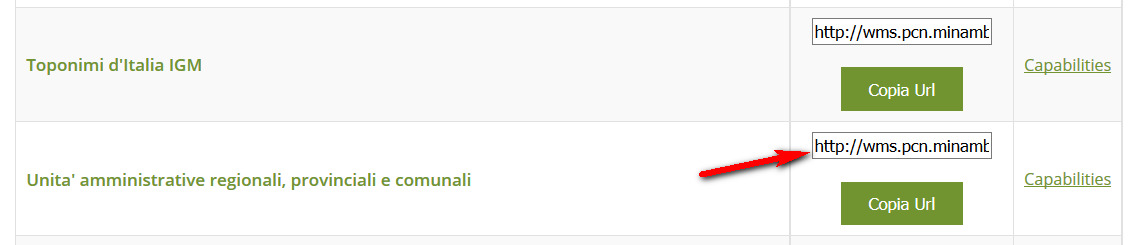
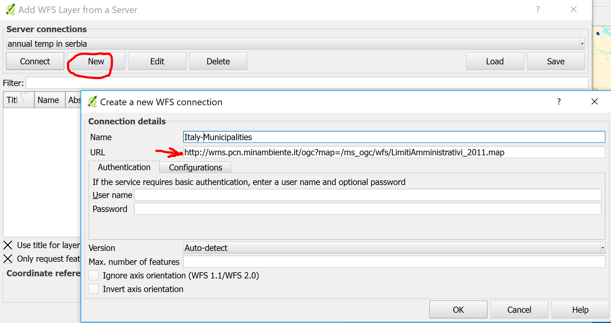
In the QGIS menu “Layer”“Add Layer”“Add WFS layer” you will get a dialogue window, click “New” and copy the URL in the input area, and give a Name to the layer
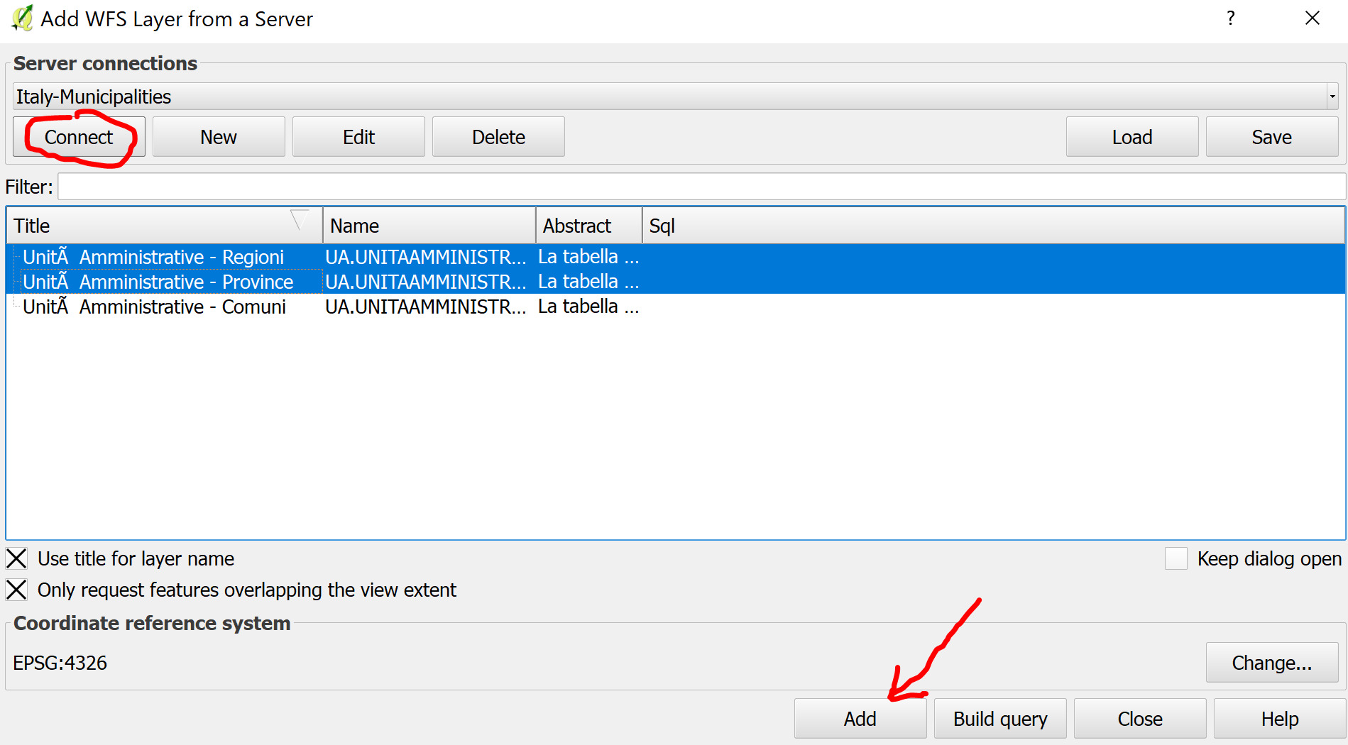
After click “ok” and “connect” from the main window. You will get three sub-layers: regions, provinces and towns – you can choose one ore more layers and then “Add” to add to project:
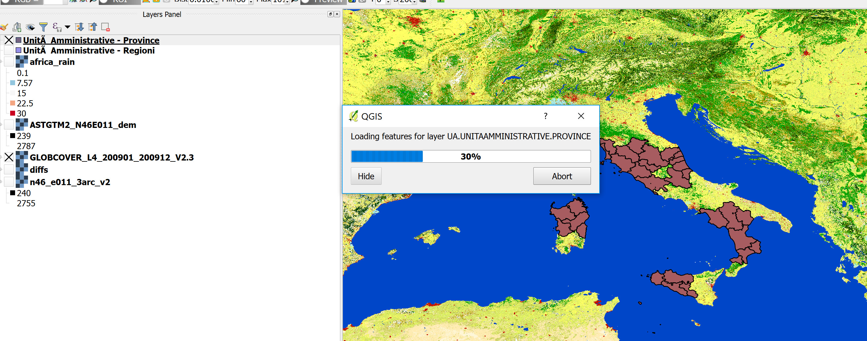
The layers will load: it might take some time depending on the size of the data, on internet connection speed and on the speed of the server providing the WFS service
NB: the same identical procedure can be used to add WMS or WCS service layers, which add raster data: QGIS menu “Layer”“Add Layer”“Add WCS layer” or “Add WMS layer”
Other OGC OWS services
https://www.qgistutorials.com/en/docs/working_with_wms.html
WMS
https://mrdata.usgs.gov/wms.html - USGS OGC Web Mapping Services
https://idt2-geoserver.regione.veneto.it/geoserver/ows - Veneto Region Styled raster
https://idt2.regione.veneto.it/gwc/service/wmts - Veneto Region orthophotos
WFS
https://mrdata.usgs.gov/wfs.html - USGS OGC Web Feature Services
https://idt2-geoserver.regione.veneto.it/geoserver/ows - Veneto Region
TMS services (OpenStreetMap)
TMS Services are a particular type of online services that provide visual maps, usually styled maps and aerial imagery (e.g. Google Maps). They are very fast to load and are used as base maps to view study area extents and provide visual information of your area.
QGIS provides two plugins to access TMS data, OpenLayers and QuickMapServices. We will use “QuickMapServices” as it is more robust. The procedure to install the plugin is the following:
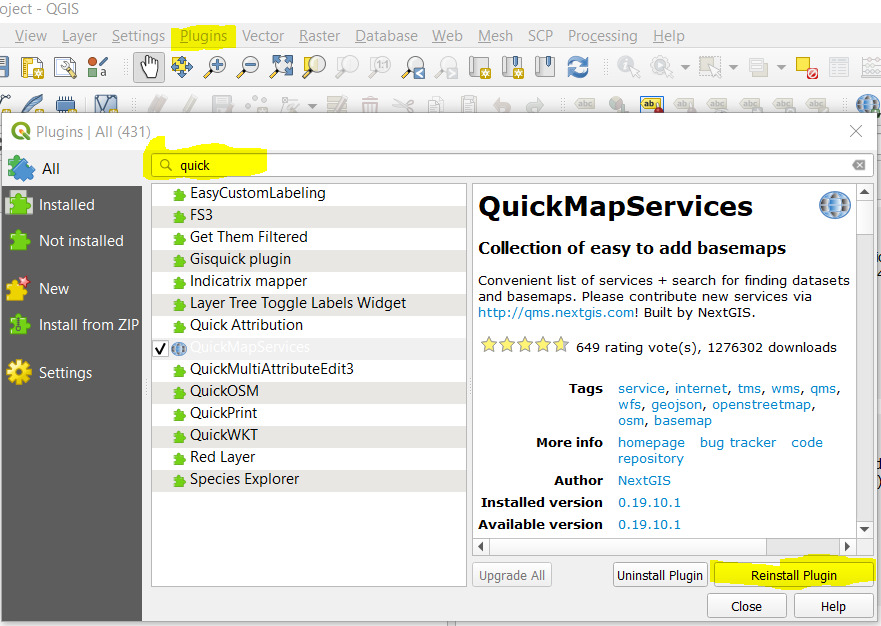
- Download the plugin “QuickMapServices” (menu “Plugins”“Manage and install plugins”). NB is you do NOT see a large list of plugins, you might not be connected to the internet or maybe QGIS has trouble connecting – to solve (i) check that internet is working (ii) close and reopen the Plugin panel window (iii) if still no plugins, restart QGIS.
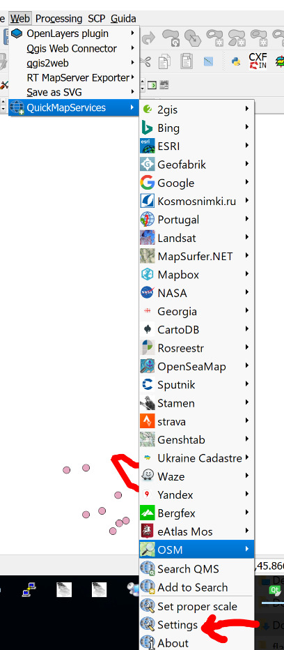
Once installed, you will see the plugin in the menu at “Web” “QuickMapServices” – you will see many available map services that can be loaded, but not all
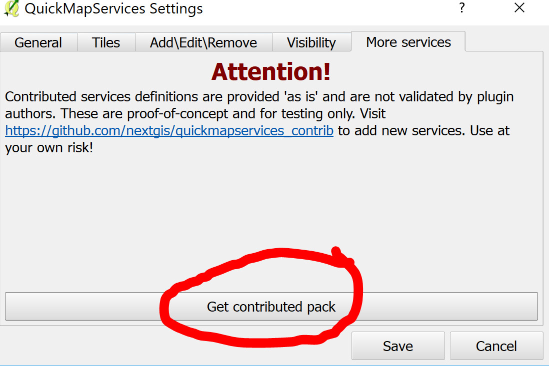
to load all services go to menu “Web”“QuickMapServices”“Settings”: from dialogue window click “More Services” “Get Contributed Pack”
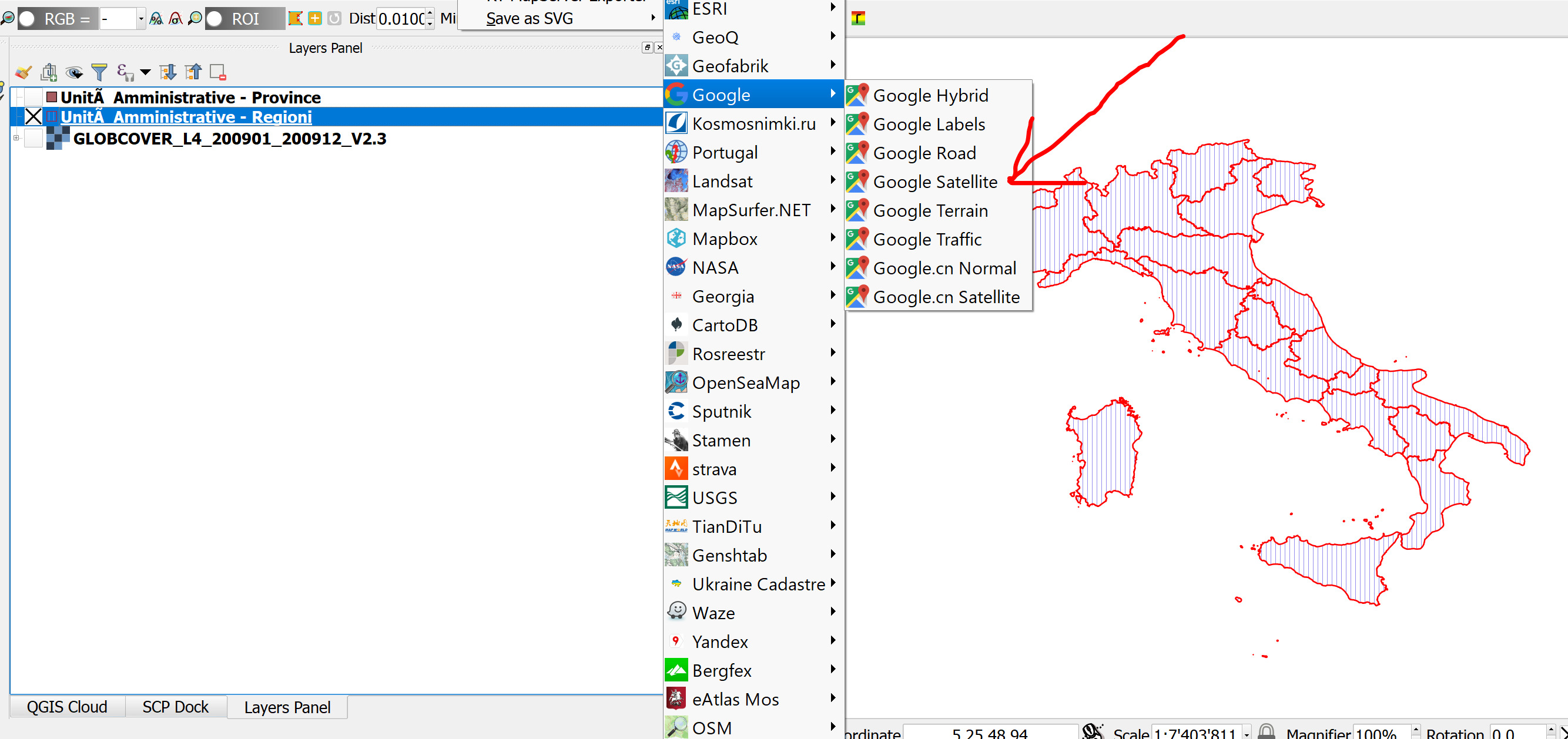
- Now from menu “Web” “QuickMapServices” you will see all available services: select “Google”“Google Satellite” you will have access to Google image database up to a resolution below 1 m in almost all of the Earth surface!!
Open Streetmap
Open StreetMap is a special type of service providing access to their data also for download. Check online tutorial Searching and Downloading OpenStreetMap Data
Exercies 3 hint: formula can be - (“Nightlights_1993@1” = 0) * “Nightlights_2003@1” - the first part creates a 0/1 result called “mask” that is then multiplied by the values from the recent image. Thus areas without lights in 1993 but with lights in 2003 will have a values > 1, whereas areas already having lights in 1993 (settlements already present) will have value 0 (we are only interested in new settlements)
Check tutorial Working with WMS Data↩︎
Check tutorial Searching and Downloading OpenStreetMap Data↩︎